


Digital Oscilloscope DS-8000 Series Various Functions
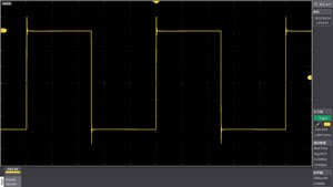
Smoothing function
Upper section:Signal where noise is superimposedInterruption:Smoothing ± 2 pointsLower section:Smoothing ± 6 pointsSimple moving average processing allows the main signal to be measured by highlighting it versus the signal with waveform distortion. From the sampling data, the average value is calculated and displayed by shifting the average value for each certain section. (which can be arbitrarily set by width)
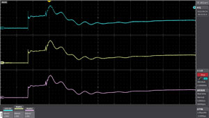
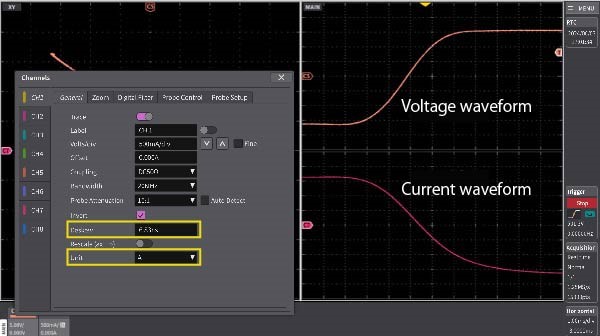
Arithmetic function
Example:Response characteristics of inductor
Upper section:Voltage change (CH1)
Middle section:Current change (CH3)
Lower section:Power change=MATH(CH1*CH3)
Using the arithmetic function, loss, impedance, etc. can be determined. In addition, as with channel input (voltage/current), MATH has a rescale function, so you can directly read the characteristic values of the device.
FFT function
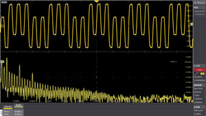
The frequency components of the input signal can be determined.
In the example in the left figure, the time axis waveform has a 500 ns period signal superimposed on the square wave signal of the 100 ns period in the upper section. In the lower section, a 10 MHz odd-order harmonic 1-3-5 order is clearly shown by FFT analysis, and a 2 MHz signal can be seen between the frequency components.
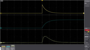
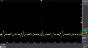
Filter function
Input signal
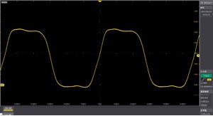
① Analog filter 20MHz
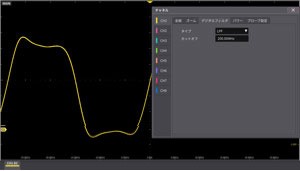
② Digital filter (LPF) 200MHz
③ Digital filter (HPF) 35MHz
For each channel, the analog filter and the digital filter can be set separately. ① Analog filter function (when 20 MHz is set) Input amplifier is band-limited to eliminate high-frequency noise. ②③ Digital filter function (when ② LPF200MHz, ③ HPF35MHz is set) The filter type and cutoff frequency can be set, and the filter function is realized by digital signal processing.
In the example, one signal can be extracted from a signal in which two frequency components are superimposed.
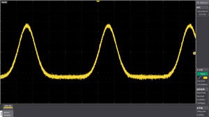
Average operation
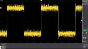
Noise-superimposed waveform (without averaging)
Averaged waveform
The left upper waveform is a superimposed waveform of noise. In the upper right waveform, the noise is reduced by averaging. Capture the trigger as a single "Then, after capturing the data for the set number of averages, stop the measurement.
High Resolution mode, Advanced High Resolution(Advanced High Resolution)
Impulse waveform with noise superimposed
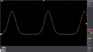
Waveforms with reduced noise in high-resolution mode
High Resolution mode When set to a sample rate lower than the highest sampling, the data captured in the highest sampling is averaged and displayed in high resolution. You can effectively increase the vertical resolution by attenuating random noise. It can also be used for single-shot signals and repeating signals, and supports up to 16 bits. Advanced High Resolution Digital processing provides higher resolution and less noise than High Resolution.
sin (x)/X interpolation
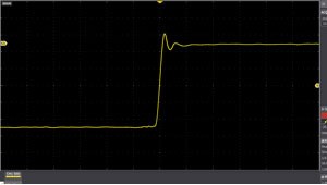
sin(x)/X interpolated waveform
Linearly interpolated waveform
In this mode, by creating interpolation data by curve fitting between acquired sampling points using sin (x)/x interpolation, the apparent sampling speed is increased and measured. Unlike equivalent sampling, it can also be used for single-shot signals.
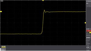
Peak detection mode
Detects and displays the maximum and minimum values that occur within the interval that is twice the set sampling period, so that peak values such as noise waveforms can be reliably understood.
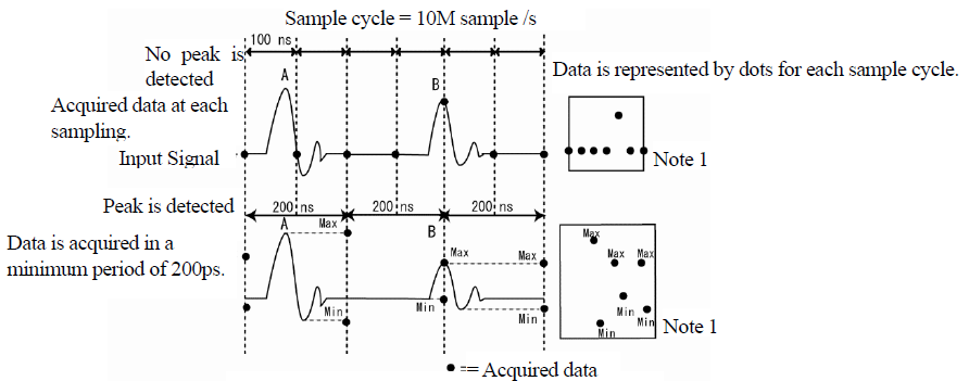
The above figure shows the capture method at the time of normal sampling (upper section) and at the time of peak detection (lower section).
If peak detection is not set, the waveform data point A in the figure may not be detected. Because it captures at 400 ps cycles independent of the sampling period, it can reliably capture phenomena that occur within the sampling period.
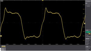
Roll sample
The waveform data is displayed in real time, and continuous waveform data is automatically scrolled from the left side of the screen to the right side. When using the maximum memory length of 120M points, very long level fluctuations of 5-50s/div can be seen continuously. The figure is an example that visually captures frequent amplitude fluctuations.
Roll operation is possible from 100 ms/div to 50 s/div with a memory length of 1.5k points as the fastest setting.
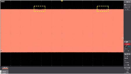
Example of checking amplitude fluctuating within 120div (120s) (time axis:1s/div)
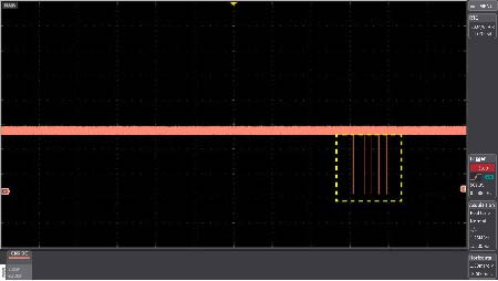
Example of peak detection of spike noise with small pulse width generated by the peak detection function (time axis:1s/div)
Cursor functions
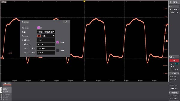
The cursor functions are Time, Amplitude, Time & Amplitude, and Value at cursor. You can move the cursor individually or track two cursors simultaneously. The figure is an example of pulse measurement with the Time & Amplitude cursor. You can view the values in the CURSOR area of the cursor menu, horizontal axis, and channel menu. Note that the cursor window of the measurement screen can also be hidden so that it does not overlap the waveform.
Split waveform display
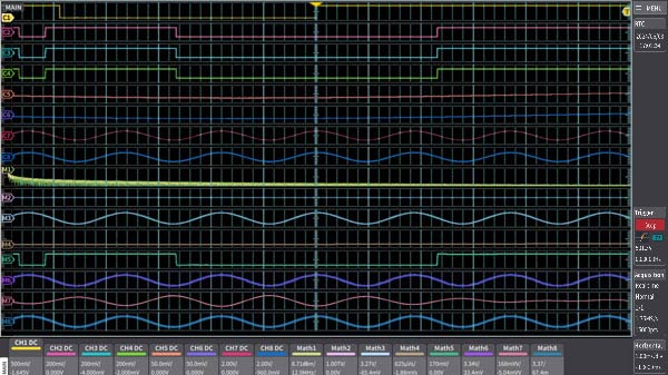
The vertical axis (amplitude) of each channel can be displayed independently. While maintaining the full scale resolution of the vertical axis, the Y-T display (vertical axis: amplitude horizontal axis: time) is displayed for up to 16 sections in the 8CH model (CH display 8 + MATH operation 8).
For example, while looking at the original waveform, you can observe integration, differentiation, smoothing, and FFT analysis at the same time.
Search function
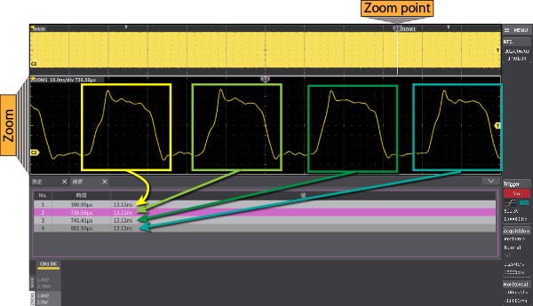
Up to 30,000 waveforms can be searched in the section that is displayed on the screen. Since the position of the waveform abnormality is easy to identify, it also leads to a reduction in debugging man-hours. The figure shows the second pulse of 13.12 ns or less, which is detected and enlarged to the lower section of the screen with the waveforms before and after.
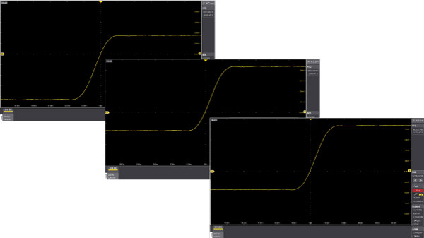
Measurement gate function
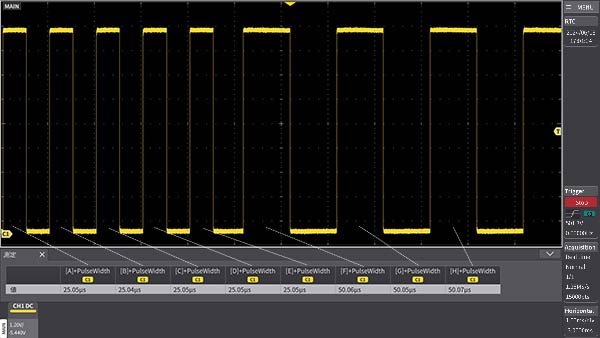
You can set each parameter operation in a specific section. As shown in the figure above, if you want to continuously check the change in pulse width at a specific timing while monitoring the waveform, you can display the respective pulse width by applying a measurement gate to each pulse. In addition, the change of the signal at different times in different channels can also be checked numerically.
Deskew function
Depending on the probe used, skewing may occur between channels. The Deskew function allows you to compensate for time differences between channels. This function is necessary for accurate loss analysis (voltage x current) and timing measurement. You can check numerically.
Sequence function/History function
The Sequence function is a high-speed trigger that allows you to set the horizontal axis sample mode to a sequence and store the data in the segmented memory, greatly reducing the data read time. The figure shows an example in which the 1/5-32,768th waveform is captured and the maximum value of each waveform is displayed.
The History function is always running in sample mode with no special settings in real-time mode. You can easily read the waveform history. The maximum number of records is 32,768 waveforms (dependent on memory). Historical data is displayed by specifying the index number of the history.
Data storage and offline analysis
By saving the measurement conditions and measurement data of the DS-8000, and later using the DS-8000 Viewer to read out the data, you can play back the waveform under different conditions, convert the waveform data to the required format (binary→ CSV format) and save it, and save the screen display in png format. To transfer long memory data to a PC, you can save via a USB3.0 storage device, or use the Ethernet or USB interface between the PC and the DS-8000.
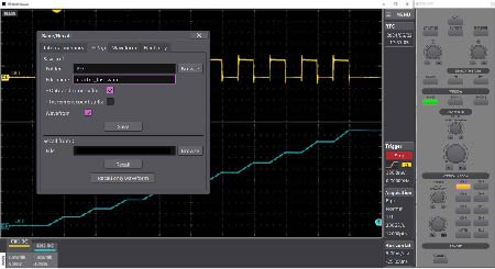
DS-8000 Viewer (Free Software)
The figure is an example of measuring current and voltage drop in the reactor.
The data is saved and the waveform is read out on the PC. Since the knobs etc. on the oscilloscope are displayed visually on the PC, you can perform analysis with the feeling of actually operating the oscilloscope.
External trigger function (factory option)
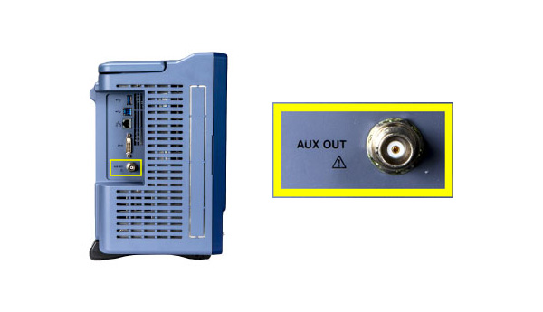
Compatible with external trigger input by selecting the AUX OUT external trigger input and the option (factory option applied at the time of shipment). You can capture the waveform using the timing of the control signal from the outside, such as system embedding.
Probe Power Connector
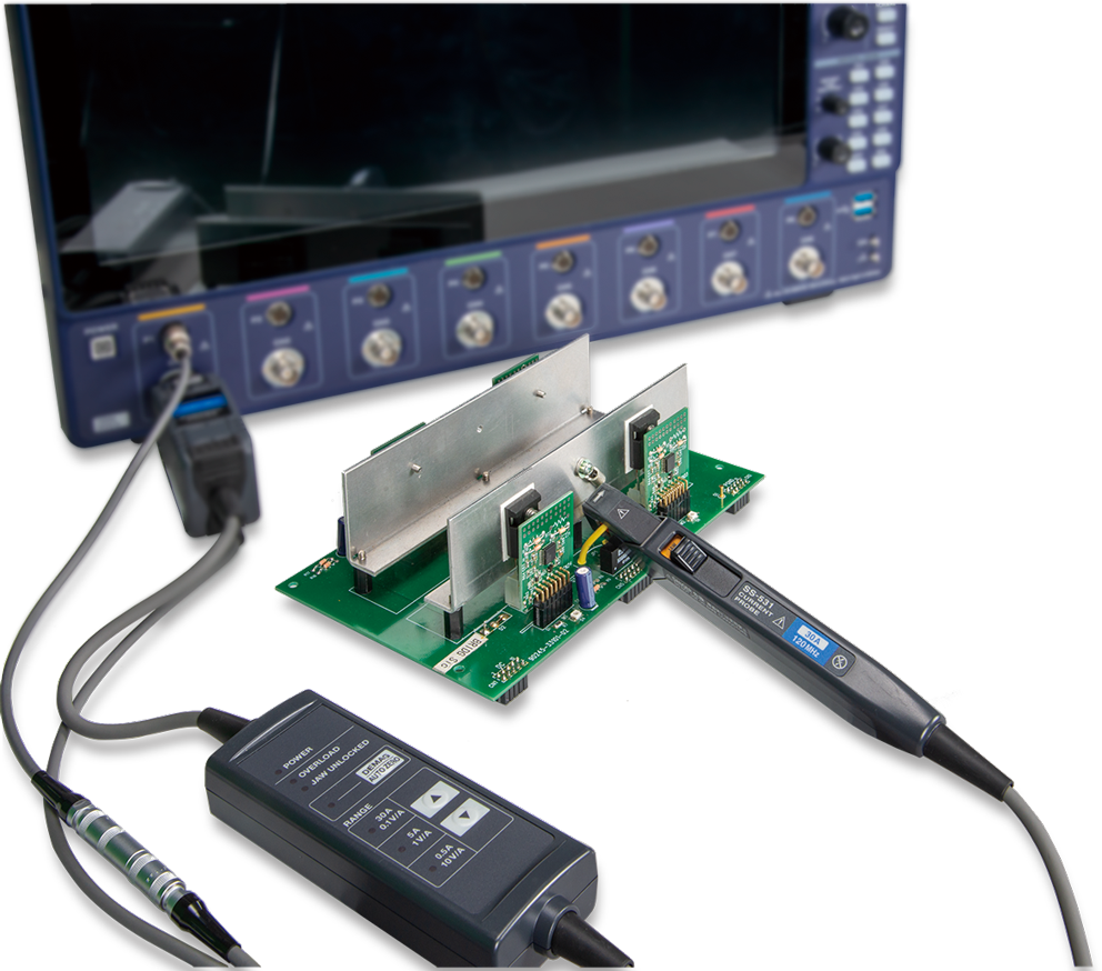
Each channel has a dedicated probe power connector.
These connectors allow to use several models of active probe without external power supply.
(Some probes require a conversion cable for usage.)
| Probe Type | Model |
|---|---|
| FET Probe | SFP-4A/5A※ |
| High Voltage Differential Probe | SS-320 |
| ON Voltage Probe | SS-350 |
| Differential Amplifier | SS-331, SS-332 |
| Current Probe | SS-240A※, SS-250※, SS-260※, SS-270※,
SS-520, SS-521, SS-530, SS-531, SS-540, SS-550, SS-560, SS-570 |
Note:Probe marked with ※ is discontinued.
Parameter for measurement
| Measure type | Measure content | Units | |
|---|---|---|---|
| Vertical (Vertical axis direction) |
Maximum | Maximum value of the waveform | V |
| Minimum | Minimum value of the waveform | ||
| Peak-Peak | Difference between maximum and minimum values | ||
| Top | Upper flat portion of the waveform | ||
| Base | Lower flat portion of the waveform | ||
| Top-Base | Difference between Top and Base (amplitude) | ||
| RMS | RMS value of waveform | ||
| Cycle RMS | RMS value of waveform per cycle | ||
| Mean | Mean value of waveform | ||
| Cycle Mean | Mean value of waveform per cycle | ||
| +OverShoot | Overshooting in waveform rise | % | |
| -OverShoot | Overshooting in waveform fall | ||
| Measure type | Measure content | Units | |
| Horizontal (horizontal axis direction) |
Transition Time | Rise / fall time of waveform | s |
| Tr 20~80% | Rise time for 20~80% of waveform | ||
| Tf 80~20% | Fall time for 80~20% of waveform | ||
| Tr 10~90% | Rise time for 10~90% of waveform | ||
| Tf 90~10% | Fall time for 90~10% of waveform | ||
| Tr Level | Rise time of waveform ( Specify the detection threshold as a real number ) | ||
| Tf Level | Fall time of waveform ( Specify the detection threshold as a real number ) | ||
| Frequency | Waveform frequency | Hz | |
| Period | Waveform period | s | |
| +Pulse Count | Number of positive pulse | - | |
| -Pulse Count | Number of negative pulse | - | |
| +Pulse Width | Width of positive pulse | s | |
| -Pulse Width | Width of negative pulse | s | |
| Duty Cycle | Waveform duty ratio ( positive pulse width / period ) | % | |
| Measure type | Measure content | Units | |
| Other | dV/dt | Slope of the rising / falling edge of the waveform | V/s |
| Integral | Integral of the waveform | Vs | |
| Integral (Absolute) | Integral of absolute value of the waveform | ||
| Integral (Positive) | Integral with only positive values of the waveform ( negative values are treated as 0 ) |
||
| Integral (Negative) | Integral with only negative values of the waveform ( positive values are treated as 0 ) |
||
| Skew (%) | Time difference between edges of waveform ( Specify the threshold for edge detection in % ) |
s | |
| Skew Level | Time difference between edges of waveform ( Specify the threshold for edge detection in real numbers ) |
||
| Phase (%) | Phase difference of the waveform ( Specify the threshold for edge detection in % ) |
Degree, Radian, % |
|
| Phase Level | Phase difference of the waveform ( Specify the threshold for edge detection in real numbers ) |
||
Examples of probes suitable for DS-8000 series
Voltage Probe
| Model | Frequency Bandwidth (MHz) |
Attenuation ratio | Maximum voltage (Vpeak) | DS-8000 Series terminator (Ω) | DS-8000 Series power supply connection | Probe power supply | |
|---|---|---|---|---|---|---|---|
| External power supply | Battery driven | ||||||
| BumbleBee (Differential) |
400 | 500:1 ~ 50:1 | ±2,000 | 50 | Not supported | PS-02, PS-03 | AP-01 |
| 500 / 400 | 50:1 ~ 5:1 | ±200 | |||||
| SS-320 (Differential) |
100 | 500:1 / 50:1 |
±1,400 | 1M | Supported | PS-25 | Not supported |
| PHV2000 | 400 | 100:1 | 4,000 | 1M | - | - | - |
| PHVS2000 | 400 | 1,000:1 | 4,000 | 1M | - | - | - |
| TETRIS 1500 | 1,500 | 10:1 | ±8V | 50 | Not supported | Standard Accessory | Not supported |
| PML711I-RO | 500 | 10:1 | 300(CATII) | 1M | - | - | - |
Current probe
■ Rogowski Coil Current Probes
| Model | Frequency Bandwidth (MHz) |
Sensitivity(mV/A) | Maximum current (Apeak) |
DS-8000 Series terminator (Ω) | DS-8000 Series power supply connection | Probe power supply | |
|---|---|---|---|---|---|---|---|
| External power supply | Battery driven | ||||||
| SS-280A Series SS-280A-H Series |
30 | 0.2 ~ 200 | 30 ~ 30,000 | 1M | Not supported | AC adapter (option) |
AA Batteries 4 pcs |
| SS-290 Series | 10 / 20 | 0.05 ~ 5 | 1,200 ~ 120,000 | 1M | |||
| SS-620 Series | 10 / 15 / 20 / 25 |
0.2 ~ 100 | 60 ~ 30,000 | 1M | |||
| SS-660 Series SS-660P Series |
30 | 5 ~ 100 | 60 ~ 1,200 | 1M | |||
| SS-680 Series | 100 | 0.1 ~ 10 | 120 ~ 12,000 | 50 | |||
■ Clamp current probe ( hole element type )
| Model | Frequency Bandwidth (MHz) |
Sensitivity(V/A) | Maximum current (Apeak) |
DS-8000 Series terminator (Ω) | DS-8000 Series power supply connection | Probe power supply | |
|---|---|---|---|---|---|---|---|
| External power supply | Battery driven | ||||||
| SS-531 | 120 | 0.1 / 1 / 10 | 30 / 5 / 0.5 | 1M | Conversion cableSS-200-IW (option) |
PS-54 (option) |
Not supported |
| SS-521 | 120 | 1 | 5 | PS-52, PS-54 (option) |
|||
| SS-550 | 100 | 0.1 | 30 | ||||
| SS-560 | 10 | 0.01 | 150 | ||||
| SS-570 | 2 | 0.01 | 500 | ||||
■ Current transformer CT Series
| Model | Frequency Bandwidth (MHz) |
Sensitivity(mV/A) | Maximum current (Apeak) |
DS-8000 Series terminator (Ω) | DS-8000 Series power supply connection | Probe power supply | |
|---|---|---|---|---|---|---|---|
| External power supply | Battery driven | ||||||
| 58, 89 Series | ~ 30 | 0.01 ~ 1 | ~ 500 | 50 | - | - | - |
| 13 Series | ~ 60 | 0.05 ~ 1 | ~ 100 | 50 | |||
Skew Calibrator
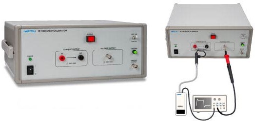
Skew calibrator IE-1360
To accurately measure the instantaneous switching loss, it is necessary to align the phase (skew) between the voltage probe and the current probe as close as possible to the actual measured voltage and current amplitude.
The skew calibrator IE-1360 is a signal generator that outputs both voltage and current pulses at the same time. It can output up to 250V and 10A so that it can calibrate with sufficient amplitude even for high voltage and high current probes used for power electronics measurement. Note that skew adjustment uses the Deskew function on the oscilloscope.
